AI Data Extraction Lab 1: When Models Remember Too Much

Neural networks are trained to learn patterns, but sometimes they learn a bit too well. Under the right conditions, ML models can memorize specific samples from their training data, and spit them back out. This has real consequences for privacy, intellectual property, and legal compliance:

• GitHub Copilot has been caught reproducing GPL-licensed code without attribution, leading to a class-action lawsuit.
• The New York Times sued OpenAI over ChatGPT reproducing entire passages of its articles.

Academic research in this space has also shown the scale of the problem:

• Carlini et al. showed that GPT-2 can be prompted into regurgitating verbatim training data, including Personally Identifiable Information (PII)
• Nasr et al. extracted over 10,000 training examples from ChatGPT for under $200

This is the first of a series of labs on data extraction attacks. My goal with these labs is to explore what’s currently possible in the realm of targeted and untargeted data extraction from large models (using resources within everyone’s reach). The main focus will be on LLMs but I might touch on other types of models if time allows. If you suspect a model was trained on some proprietary data and want to check whether it ended up memorizing it, I am planning to cover a range of techniques, from basic to advanced.

Models can “memorize”

The goal of this first lab is simple: building an intuition that models, under the right settings, can “memorize” samples from their training data. But what does memorization even mean?

At their core, neural networks are statistical models designed to capture data distributions. In this context, what does it even mean for a model to “memorize” some data?

• Carlini et al. define memorization in terms of extractability: a string s is considered memorized if you can find a prompt p such that the model reproduces s verbatim when given p as input.
• Memorization is also commonly measured via membership inference: given a sample, can you determine whether it was part of the model’s training data? (e.g. Mireshghallah et al.)
• Zhang et al. introduced the concept of counterfactual memorization: how much would a model’s predictions change if a specific document were removed from the training data?

In practice, there are multiple ways to look at memorization, and all are complementary and relevant under different threat models.

Storing data

But how much data can a model actually store? Morris et al. found that GPT-style architectures have a capacity of approximately 3.6 bits per parameter. To put that in perspective, a 1-billion parameter model could in principle store around 450 MB of raw data. The best text compression algorithms can get close to a ~10x compression ratio, so if a model stores information as efficiently as a good compressor, a 1-billion parameter LLM could in principle retain the equivalent of ~4.5 GB of uncompressed text.

Training sets can be orders of magnitude larger than models storage capacity (e.g. The Pile’s size is > 800GB). Clearly, models are generally unable to store the entirety of their training data verbatim, and memorization must be limited to a small subset of samples.

Interestingly Maini et al. show that often memorization isn’t spread uniformly across a network, but concentrated in a small set of neurons. Carlini et al. found that memorization grows logarithmically with model size. In their experimental setting they observed that:

a ten fold increase in model size corresponds to an increase in memorization of 19 percentage points

They also observed a similar relationship with respect to the number of times a sample is duplicated in the training data.

There’s also a connection between the structure of the data and how easily it gets memorized. Recent work on data compressibility and memorization shows that more compressible (i.e. more structured, more predictable) data is easier for models to memorize. However, if we change our frame of reference to counterfactual memorization this relationship changes and models seem to memorize better “intermediate simplicity” samples rather than easy ones.

So, the answer to our initial question: “how much data can a model actually store?” is “it’s complicated”.

Overfitting & model size

Memorization is often associated with overfitting. While this is not always the case, overfitting can certainly play a role. To get a sense of this, let’s start by playing with some toy models.

The widget below lets you train a simple neural network. The goal of the network is to classify points in space into one of two classes. Ideally, we’d want the classifier to generalize the distribution and ignore outliers. Try training the model using a large hidden width (e.g. 20), and then a very small width (e.g. 2). You should observe how larger models tend to overfit the training data more easily, clearly storing within their “memory” the approximate location of outliers. Similarly, regardless of size, training for more epochs on the same data is more likely to cause the model to overfit.

Memorization at first sight

In the previous example, we saw the model overfitting the data after many training iterations. But under the right conditions, models can leak training data after surprisingly few exposures. The widget below lets you train a character-level GRU language model on a small synthetic dataset.

The dataset used to train the model contains 200 unique sequences (aka words) of 5 letters, where each letter is picked from an alphabet of 16 characters. In principle our model should learn to generate 5-letter words drawing from a space of $16^5$ possible combinations. In practice our dataset is designed to contain predictable patterns so that learning a sequence facilitates learning of other similar (but distinct) entries. In other words, we expect learning to transfer and ease memorization. You can inspect the dataset here.

As training progresses, the widget shows which words the model assigns the highest probability to, along with how many times each word was encountered during training.

Pay attention to the “seen” counts. You should notice that words seen only once or twice can quickly climb to the top of the probability rankings: the model memorizes them despite their rarity. Try experimenting with the hidden width: a wider model has more capacity to store these low-frequency words, while a narrower one is forced to generalize. Similarly, smaller batch sizes make individual rare words more impactful during gradient updates, increasing memorization.

Memorization in Real LLMs

So far we’ve seen memorization in toy models. Can the same thing happen at scale, with real LLMs trained on internet-scale data? For this we will use an approach inspired from “Quantifying Memorization Across Neural Language Models” by Carlini et al..

We will probe Pythia, a suite of open-source language models trained on The Pile, by feeding it prefixes drawn directly from its training data and checking whether it can reproduce what originally followed. Because The Pile is public and Pythia’s training data is documented, we can compare the model’s output to the ground truth. We will test two model sizes (Pythia 1.4B and Pythia 410M) and vary the prompt length to observe how both factors affect memorization.

Setup

The configuration block defines the two Pythia checkpoints we’ll compare, the dataset to probe, and the key experimental parameters — prompt lengths, number of samples, and generation length.

import heapq
import random
from pathlib import Path
from typing import Optional

import matplotlib.pyplot as plt
import torch
from datasets import load_dataset
from tqdm.auto import tqdm
from transformers import AutoModelForCausalLM, AutoTokenizer

TARGET_MODEL_NAME = "EleutherAI/pythia-1.4b"  # Main model whose continuations we evaluate
COMPARISON_MODEL_NAME = "EleutherAI/pythia-410m"  # Smaller companion model evaluated with the same prompts
DEVICE = "cuda" if torch.cuda.is_available() else "cpu"
MODEL_DTYPE = torch.float16 if DEVICE == "cuda" else torch.float32  # Lower GPU memory usage on CUDA

PILE_DATASET_REPO = "EleutherAI/the_pile_deduplicated"  # Public deduplicated Pile corpus
PILE_DATASET_SPLIT = "train"
PILE_TEXT_KEY = "text"

GENERATION_LENGTH = 50  # Number of tokens the model must continue after each prompt
N_SAMPLES = 5000  # Number of valid prompt/continuation pairs collected per prompt length
EVAL_BATCH_SIZE = 8  # Batch size used during generation
PROMPT_SIZES = [50, 150, 450, 950]  # Prefix lengths evaluated for each model
TOP_EXAMPLES = 100  # Number of matches shown in the qualitative summary
RANDOM_SEED = 0  # Shared seed for reproducible dataset shuffling and span sampling
SHUFFLE_REFERENCE_DATA = True  # Approximate uniform sampling instead of always using the first streamed documents
SHUFFLE_BUFFER_SIZE = 10000  # Streaming shuffle buffer size for Hugging Face iterable datasets
SAMPLE_RANDOM_SPANS = True  # Sample a random contiguous span from each document instead of always using the document prefix

MAX_PROMPT_SIZE = max(PROMPT_SIZES)  # Longest prefix; all prompts are right-aligned to this boundary
MAX_SEQUENCE_TOKENS = MAX_PROMPT_SIZE + GENERATION_LENGTH  # Sequence length collected once, then sliced for every prompt length.

Then load both checkpoints and put them in eval mode:

tokenizer = AutoTokenizer.from_pretrained(TARGET_MODEL_NAME)
if tokenizer.pad_token is None:
    tokenizer.pad_token = tokenizer.eos_token

torch.manual_seed(RANDOM_SEED)

target_model = AutoModelForCausalLM.from_pretrained(
    TARGET_MODEL_NAME,
    torch_dtype=MODEL_DTYPE,
).to(DEVICE)
comparison_model = AutoModelForCausalLM.from_pretrained(
    COMPARISON_MODEL_NAME,
    torch_dtype=MODEL_DTYPE,
).to(DEVICE)

for loaded_model in (target_model, comparison_model):
    loaded_model.eval()
    loaded_model.config.pad_token_id = loaded_model.config.eos_token_id

Step 1: Sample prompts from the training data

We stream EleutherAI/the_pile_deduplicated from Hugging Face and collect token sequences of a fixed length. Each sequence is later split into a prompt (the prefix we feed to the model) and a continuation (the ground truth we want to recover).

The dataset is shuffled before streaming so we get a representative cross-section of documents rather than always pulling from the same source files:

def load_reference_dataset_stream():
    dataset_stream = load_dataset(
        PILE_DATASET_REPO,
        split=PILE_DATASET_SPLIT,
        streaming=True,
    )

    if SHUFFLE_REFERENCE_DATA:
        dataset_stream = dataset_stream.shuffle(
            seed=RANDOM_SEED,
            buffer_size=SHUFFLE_BUFFER_SIZE,
        )

    return dataset_stream

Rather than always taking the first tokens of each document, we sample a random span from within it (this avoids biasing toward document openings, which tend to be more predictable regardless of memorization). collect_reference_sequences iterates the stream and assembles N_SAMPLES token spans of length MAX_SEQUENCE_TOKENS:

def sample_random_span(
    token_ids: list[int],
    sequence_length: int,
    rng: random.Random,
) -> Optional[list[int]]:
    if len(token_ids) < sequence_length:
        return None

    if not SAMPLE_RANDOM_SPANS or len(token_ids) == sequence_length:
        start_index = 0
    else:
        start_index = rng.randrange(len(token_ids) - sequence_length + 1)

    return token_ids[start_index : start_index + sequence_length]


def collect_reference_sequences(
    n_samples: int,
    sequence_length: int,
) -> list[list[int]]:
    sampled_sequences = []
    rng = random.Random(RANDOM_SEED)

    for row in load_reference_dataset_stream():
        token_ids = tokenizer.encode(row.get(PILE_TEXT_KEY, ""), add_special_tokens=False)
        span = sample_random_span(token_ids, sequence_length, rng)
        if span is None:
            continue
        sampled_sequences.append(span)

        if len(sampled_sequences) >= n_samples:
            break

    if len(sampled_sequences) < n_samples:
        raise ValueError(
            f"Collected only {len(sampled_sequences)} sequences of length {sequence_length} "
            f"from the configured reference data, but expected {n_samples}."
        )

    return sampled_sequences

All prompts are right-aligned to the same boundary: for a given prompt_size, the prompt covers the prompt_size tokens immediately before MAX_PROMPT_SIZE, so the continuation to predict is the same fixed GENERATION_LENGTH tokens regardless of prompt length. This means we’re testing whether more context helps reproduce the same target, rather than comparing different parts of the sequence across conditions.

def build_prompt_batch(
    reference_sequences: list[list[int]],
    prompt_size: int,
) -> list[list[int]]:
    prompt_start = MAX_PROMPT_SIZE - prompt_size
    return [seq[prompt_start : prompt_start + prompt_size] for seq in reference_sequences]

Step 2: Generate and evaluate

To measure how close the model’s output is to ground truth we use edit distance at the token level: the minimum number of insertions, deletions, and substitutions required to transform the predicted sequence into the reference one. An edit distance of 0 means verbatim reproduction.

def edit_distance(predicted_ids, actual_ids):
    actual_length = len(actual_ids)
    predicted_length = len(predicted_ids)
    dp = list(range(predicted_length + 1))

    for actual_index in range(1, actual_length + 1):
        previous_diagonal = dp[0]
        dp[0] = actual_index

        for predicted_index in range(1, predicted_length + 1):
            previous_value = dp[predicted_index]
            if actual_ids[actual_index - 1] == predicted_ids[predicted_index - 1]:
                dp[predicted_index] = previous_diagonal
            else:
                dp[predicted_index] = 1 + min(
                    previous_diagonal,
                    dp[predicted_index],
                    dp[predicted_index - 1],
                )
            previous_diagonal = previous_value

    return dp[predicted_length]

evaluate_prompt_examples runs greedy decoding (do_sample=False) over all prompts in batches, then scores each continuation immediately:

def evaluate_prompt_examples(
    model,
    prompt_batches,
    actual_batches,
    label: str,
    batch_size: int = EVAL_BATCH_SIZE,
):
    results = []
    prompt_size = len(prompt_batches[0])

    progress_bar = tqdm(
        range(0, len(prompt_batches), batch_size),
        desc=label,
        unit="batch",
        leave=False,
    )

    for start in progress_bar:
        batch_prompts = prompt_batches[start : start + batch_size]
        batch_actuals = actual_batches[start : start + batch_size]

        input_ids = torch.tensor(batch_prompts, device=DEVICE)
        attention_mask = torch.ones_like(input_ids)

        with torch.no_grad():
            outputs = model.generate(
                input_ids=input_ids,
                attention_mask=attention_mask,
                max_new_tokens=GENERATION_LENGTH,
                do_sample=False,
                pad_token_id=tokenizer.pad_token_id,
            )

        for batch_index in range(len(batch_prompts)):
            predicted_ids = outputs[batch_index, prompt_size:].tolist()
            actual_ids = batch_actuals[batch_index]
            results.append(
                {
                    "actual": tokenizer.decode(actual_ids),
                    "predicted": tokenizer.decode(predicted_ids),
                    "distance": edit_distance(predicted_ids, actual_ids),
                }
            )

    return results

Step 3: Sweep prompt lengths and model sizes

Now let’s wire the pieces together. The reference sequences are collected once at the maximum length; the ground-truth continuation is always the same last GENERATION_LENGTH tokens. For each prompt length, we build the right-aligned prompt batch and evaluate both models:

experiment_results = {}
reference_sequences = collect_reference_sequences(N_SAMPLES, MAX_SEQUENCE_TOKENS)
actual_batches = [seq[MAX_PROMPT_SIZE:MAX_SEQUENCE_TOKENS] for seq in reference_sequences]

for prompt_size in PROMPT_SIZES:
    prompt_batches = build_prompt_batch(reference_sequences, prompt_size)

    for model, model_name, model_key in [
        (target_model, TARGET_MODEL_NAME, "target"),
        (comparison_model, COMPARISON_MODEL_NAME, "comparison"),
    ]:
        label = f"{model_name} — prompt size {prompt_size}"
        results = evaluate_prompt_examples(model, prompt_batches, actual_batches, label=label)
        experiment_results[(model_key, prompt_size)] = results
        print_summary(results, label)

Computing edit distances for 5,000 samples across eight conditions takes a while. The Colab at the end of the post has the full output, but you can start with a smaller N_SAMPLES (e.g. 500) to verify your setup first.

Results

Running the full experiment produces the following verbatim reproduction rates (edit distance = 0):

Prompt tokens	Pythia 1.4B	Pythia 410M
50	1.06% (53 / 5000)	0.56% (28 / 5000)
150	1.74% (87 / 5000)	1.22% (61 / 5000)
450	2.80% (140 / 5000)	2.20% (110 / 5000)
950	3.64% (182 / 5000)	2.68% (134 / 5000)

Widening the threshold to near-verbatim reproductions produces even higher rates: for Pythia 1.4B at prompt size 950, 4.54% of samples fall within edit distance ≤ 2, and 5.32% within edit distance ≤ 5. These are samples where the model gets almost everything right, differing from the original by only a handful of tokens.

Let that sink in: more than 5% of randomly sampled training spans are memorized almost verbatim by the model.

Caveats
First, we haven’t controlled for how much the prompt itself predicts its continuation, some spans may be reproducible regardless of memorization.
Second, and perhaps more surprisingly, the model cannot actually have memorized 5% of the training corpus by volume: using the 3.6 bits/parameter capacity from earlier, Pythia 1.4B can store at most $\frac{1.4 \times 10^9 \times 3.6}{8} \approx 630\,\text{MB}$ of raw data, under 0.1% of the ~800 GB training set (or ~1% if we account for text compression). The two numbers are reconciled by the fact that memorized content (i.e. boilerplate, repeated strings) is massively duplicated in the training data, so a small memorized pool hits a disproportionate share of random samples.

Two clear patterns emerge from the data.

Longer context leads to more memorization. With a 50-token prompt, the 1.4B model reproduces 1.06% of continuations verbatim. With a 950-token prompt that figure rises to 3.64%, more than tripling the rate.

Larger models memorize more. At every prompt length, Pythia 1.4B outperforms Pythia 410M on exact matches. More parameters give the model more capacity to retain specific training examples, which aligns with the logarithmic scaling relationship discussed earlier.

The edit distance distribution for Pythia 1.4B at prompt size 950 makes the memorization effect visually clear:

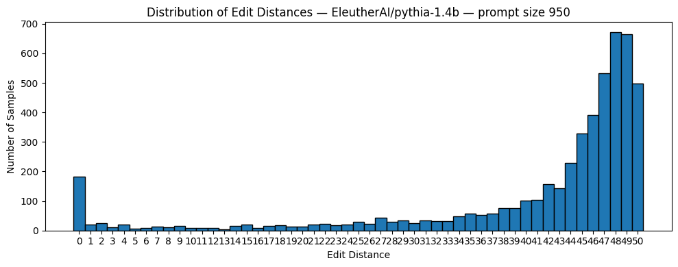Distribution of token-level edit distances for Pythia 1.4B at prompt size 950 (5,000 samples).

The distribution has a sharp spike at distance 0, a sudden drop at distance 1, and then a gradual rise across higher distances where the model is essentially generating freely. There are two distinct populations of samples: those the model has memorized and those it has not.

The top-ranked verbatim reproductions are rich in boilerplate text: GPL license headers, copyright notices, and repetitive structured data:

Original : * the Free Software Foundation; either version 2 of the License, or
           * (at your option) any later version.
           * This program is distributed in the hope that it will be useful,
           * but WITHOUT ANY WARRANTY; ...
Predicted: * the Free Software Foundation; either version 2 of the License, or
           * (at your option) any later version.
           * This program is distributed in the hope that it will be useful,
           * but WITHOUT ANY WARRANTY; ...

This is compatible with our expectations: highly structured, frequently duplicated text is the easiest for models to encode and retrieve.

Even among the 50-token prompt results, virtually every run surfaces reproductions of high-entropy and/or sensitive data: UUIDs, file paths, cryptographic hashes, email addresses, phone numbers.

Original : Release|Windows Mobile 5.0 Pocket PC SDK (ARMV4I)\n		{8559448A-4279-495E-B22B-CC35E87247E7}.Release|Windows Mobile 5.0
Predicted: Release|Windows Mobile 5.0 Pocket PC SDK (ARMV4I)\n		{8559448A-4279-495E-B22B-CC35E87247E7}.Release|Windows Mobile 5.0

The complete notebook with full output is available here: Open in Google Colab

Wrapping up

Hope you enjoyed this first lab! We started with some intuition-building on toy models and ended up extracting memorized training data from a real 1.4 billion parameter LLM, which I think is pretty cool.

The main takeaways are fairly simple: models do memorize, bigger models memorize more, and giving them more context makes it easier to trigger. The effect is most visible on highly structured and repetitive text, but it also surfaces potentially sensitive data. The former is primarily a copyright concern; the latter is a privacy one, and it shows up at every model size and prompt length we tested.