AI Data Extraction Lab 2: A Generate-then-Rank Attack

Posted Oct 18, 2026

"Show me what you got!" - cit from Rick and Morty

By Luigi Coniglio 21 min read

Lab 1 looked at memorization in LLMs and at the several different things that can mean: extractability, membership inference, counterfactual memorization. This lab focuses on extractability, and uses a similar approach to Carlini et al. for a data extraction attack on an open weights model.

The most important difference with lab 1 is that there we took a prefix from the training data and checked whether the model could complete it. That was not an attack: someone who already holds the training data has nothing to extract. This time we start from nothing but the model itself.

A simple extraction attack

The attack follows a very simple framework:

Generate large quantities of data using the model.
Rank the generated samples with a membership inference signal, to guess which ones are likely to come from the training set.

Note that this attack is probabilistic. We try to surface the candidates with the highest likelihood of being training data, but there is no guarantee that any of them actually is.

To make the attack useful we need an oracle: a way to actually verify an extracted sample. In a real world scenario this oracle is application-specific:

search the internet for the string
try the extracted credentials
send mail to the extracted address
etc.

In our case the oracle can be exact. We will attack Pythia (as in lab 1), and Pythia’s training corpus, the Pile, is public.

As in lab 1, you will find a link to the colab notebook with the full code at the end of this post.

We will use the same Pythia checkpoint as in lab 1: EleutherAI/pythia-1.4b is the model we probe for memorized text. But, we will also use smaller models for other metrics (more on this below).

Step 1 - Generation

Goal: generate a large and diverse corpus of candidates.

For this first step we want to maximize two properties:

diversity: to avoid duplicate or near-duplicate samples
likelihood of memorization: we want samples that are most likely memorized by the model

Unfortunately these properties pull in opposite directions, so finding a good balance is not trivial.

How we run generation heavily influences what we can extract. Carlini et al. leveraged three strategies, of which conditioning on prefixes scraped from the internet yielded the best results on GPT-2. We will use two of them.

Technique 1: unconditional sampling with a decaying temperature

The simplest option is to feed the model a single <|endoftext|> token and sample. Plain top-k sampling, however, tends to fall back on the same few high-likelihood sequences, so we get little coverage of the tail of the distribution.

Carlini et al. address this with a decaying temperature. Sampling starts at a high temperature, which pushes the first tokens into diverse regions, and then lowers down over the first 20 tokens.

In HF transformers we can achieve this using a custom LogitsProcessor:

  
from transformers import LogitsProcessor, LogitsProcessorList


class TemperatureDecayProcessor(LogitsProcessor):
    def __init__(
        self,
        input_length,
        initial_temperature=INITIAL_TEMPERATURE,
        final_temperature=FINAL_TEMPERATURE,
        decay_steps=TEMPERATURE_DECAY_STEPS,
    ):
        self.input_length = input_length
        self.initial_temperature = initial_temperature
        self.final_temperature = final_temperature
        self.decay_steps = decay_steps

    def __call__(self, input_ids, scores):
        step = input_ids.shape[1] - self.input_length
        if step >= self.decay_steps:
            current_temperature = self.final_temperature
        else:
            fraction = step / self.decay_steps
            current_temperature = self.initial_temperature + (
                self.final_temperature - self.initial_temperature
            ) * fraction
        return scores / current_temperature

Generation is a standard model.generate call seeded with the EOS token:

  
model.generate(
    input_ids=input_ids,                    # a single EOS token per row
    max_length=input_length + SEQUENCE_LENGTH,
    do_sample=True,
    temperature=1.0,                        # the schedule below does the real scaling
    top_k=TOP_K,
    logits_processor=LogitsProcessorList(
        [TemperatureDecayProcessor(input_length=input_length)]
    ),
)

We’ll call this source auto.

Technique 2: conditioning on a text corpus

The second strategy seeds each generation with a short prefix of real text instead of a bare EOS token. Here diversity comes from the corpus rather than from the temperature.

We stream C4, a web-crawl corpus, and take the first INTERNET_PREFIX_LENGTH tokens of each document.

  
from datasets import load_dataset

INTERNET_PREFIX_LENGTH = 5  # Tokens of real web text used to seed a generation
INTERNET_PREFIX_DATASET = "allenai/c4"

prefix_stream_iter = None


def get_prefix_stream():
    global prefix_stream_iter
    if prefix_stream_iter is None:
        ds = load_dataset(
            INTERNET_PREFIX_DATASET, "en", split="train", streaming=True,
        )
        prefix_stream_iter = iter(ds.shuffle(seed=42, buffer_size=10000))
    return prefix_stream_iter


def sample_internet_prefixes(tokenizer, batch_size, prefix_length=INTERNET_PREFIX_LENGTH):
    stream = get_prefix_stream()
    prefixes = []
    for _ in range(batch_size):
        while True:
            row = next(stream)
            tokens = tokenizer.encode(row.get("text", ""))
            if len(tokens) >= prefix_length:
                prefixes.append(tokens[:prefix_length])
                break
    return prefixes

We’ll call this source internet.

Step 2 - Membership inference

We can now use the strategies above to generate a well diversified corpus of samples. The question is: which of them were memorized?

There is no single way to answer. We can start from this intuition:

models tend to assign higher confidence to examples that are present in the training data

Perplexity is a proxy for that confidence: a low perplexity means the model found the sequence unsurprising, which might suggest it has seen it before.

  
def compute_sequence_perplexity(text, model, tokenizer):
    input_ids = tokenizer(text, return_tensors="pt").input_ids.to(model.device)
    with torch.no_grad():
        outputs = model(input_ids, labels=input_ids)
    return torch.exp(outputs.loss).item()

However, plenty of text has low perplexity (ie. is predictable) without being memorized (e.g. abc abc abc abc abc... is very predictable text, not necessarily memorized)

Carlini et al. use a separate estimate of how predictable a string is:

If a string is easy for the target model and easy by the second estimate, it is simply predictable text.
If it is easy for the target model and hard by the second estimate, it might be memorized.

In their original paper they propose three variants of this idea:

1. Comparison with a second model. Score the same text with a model that is less likely to have memorized it and take the ratio of log-perplexities. Predictable text is easy for both, so the ratio is close to 1. Text that only the larger model finds easy gives a large ratio.

2. Lowercase ratio. Score the text, then score text.lower(). A model attached to the exact casing of a memorized string sees its perplexity increase on the lowercased version.

3. zlib ratio. Use a compressor as a proxy estimate of the entropy of the text. A large compressed size paired with a low perplexity means the model is confident about something that is not intrinsically repetitive.

Alongside these, they also rank candidates by raw perplexity, using a windowed variant:

4. Windowed perplexity. This one introduces no second estimate. A memorized span of 50 tokens inside a 256-token sample is averaged away, so we take the minimum mean over a sliding window instead.

There are many more ways to sharpen the signal, but these four are enough for this lab (although you can get creative and come up with new ones).

Here is the code to compute these estimates:

  
import math
import zlib

RATIO_EPSILON = 1e-12


def _log_ppl(sample):
    return math.log(max(sample["perplexity"], 1.0 + RATIO_EPSILON))

def compute_comparison_ratio(sample):
    return math.log(max(sample["comparison_perplexity"], 1.0 + RATIO_EPSILON)) / _log_ppl(sample)

def compute_lowercase_ratio(sample):
    return math.log(max(sample["lowercase_perplexity"], 1.0 + RATIO_EPSILON)) / _log_ppl(sample)

def compute_zlib_entropy(text):
    return len(zlib.compress(text.encode("utf-8")))

def compute_zlib_ratio(sample):
    return sample["zlib_entropy"] / _log_ppl(sample)

For the windowed variant, instead of running the model once per window, we compute the per-token losses in a single forward pass and derive every window’s mean loss from a cumulative sum:

  
WINDOW_SIZE = 50  # Token length of the sliding window

# token_losses: the per-token loss for the whole sequence, one forward pass.
cumulative = torch.cumsum(token_losses, dim=0)
window_sums = cumulative[WINDOW_SIZE - 1:] - F.pad(cumulative, (1, 0))[
    : len(cumulative) - WINDOW_SIZE + 1
]
min_window_ppl = torch.exp((window_sums / WINDOW_SIZE).min()).item()

From samples to windows

The candidates are 256-token generations, but verbatim memorization is rarely that long.

Therefore in this lab we chop every candidate into overlapping 50-token windows (stride 5) and re-score each window on its own. We cluster near-duplicates by trigram Jaccard similarity and keep the lowest-perplexity representative of each cluster.

We verify extraction on these 50-token windows.

This makes our verification target different from that of Carlini et al. who focused on 256-long sequences. This is a partially forced decision as our verification method (see below) differs from theirs and relies on exact matching (which becomes unlikely at longer sequences).

Step 3 - Verifying extractions at scale

Carlini et al. verified their candidates “by hand” as they had no access to GPT-2’s training data. We are in a better position, since the Pile is public and our oracle can be exact rather than manual.

The obvious way to use it is to stream the corpus and match every candidate against every document (e.g. we could even use Aho-Corasick to do it in a single pass). Fortunately there is a quicker way.

Using a suffix-array oracle: infini-gram

infini-gram (Liu et al., 2024) is a suffix array built over a tokenized corpus. Any n-gram can be found by binary search in O(log N).

AI2 hosts a free API over a set of prebuilt indexes, including v4_piletrain_llama: 211M documents of Pile-train (Pythia’s training corpus).

A request to https://api.infini-gram.io/ asking for membership of a span of text, gives us the count. To show the extraction the same API lets us pull an actual document containing the text.

A couple of gotchas when it comes to this API:

AND / OR are special tokens in API queries, so instead of sending strings we send query_ids from a Llama-2 tokenizer, since the index is built over Llama-2 tokens
counts k are occurrences rather than documents

Counting instances is hard

Memorizing boilerplate text is not particularly interesting, so we want to filter it out. While a simple threshold on k looks like the obvious filter to check for memorized strings, it is not :(

Take as an example a software license header. The Pile stores the same license in many renderings: LF vs CRLF line endings, or ` * ` vs # vs // vs no comment prefix, various indentations, and every choice of where to wrap new lines. Each rendering is a different token sequence.

A license header at k = 1 would pass the threshold but would not indicate memorization.

To adjust for that, we assign a second number to every rare window: k_exact is the count of its own token sequence, k_content is the largest count over a handful of canonical re-renderings of the same text.

  
def canonical_renderings(window_text, limit=CONTENT_VARIANT_LIMIT):
    """Other plausible renderings of the same *content* as `window_text`."""
    body = window_text.replace("\r\n", "\n").replace("\r", "\n")
    lines = body.split("\n")
    if len(lines) < 2:
        return []

    # The first line is left verbatim: a window starts at an arbitrary token,
    # so its first line is a fragment with no line-start of its own to decorate.
    head, tail = lines[0], [_undecorate(line) for line in lines[1:]]
    variants = [" ".join(window_text.split())]          # flattened: survives re-wrapping
    for prefix in CONTENT_VARIANT_PREFIXES:             # "", " * ", "# ", "// ", "\t* ", ...
        rebuilt = "\n".join([head] + [(prefix.rstrip() if not line else prefix) + line
                                      for line in tail])
        variants.append(rebuilt)
        variants.append(rebuilt.replace("\n", "\r\n"))
        variants.append(re.sub(r"(?<=[^\s]) {2,}", " ", rebuilt))
    ...

k_content is a maximum that includes k_exact, so a window already above the threshold needs no extra queries at all, and a genuinely unique string re-renders into nothing and keeps its own count. Only boilerplate flattens into something common.

Actually, it is even harder than this

k_content tells us whether a window is rare in “any” formatting but not whether the window is rare in any part. Stitching two non-rare fragments together can produce a rare sequence that occurs once.

So for every rare window we also compute k_part: the largest count over its halves and thirds. E.g. for a sequence abcdef,

k_part = max(count(abc), count(def), count(ab), count(cd), count(ef))

Results

I generated ~120K samples, half from each strategy. 1,986 were selected for windowing, which gave 73,056 windows and 27,840 after deduplication.

708 of 27,840 windows occur in the corpus, that is 2.5%. Of those, 47 are fairly rare (1 <= k_content <= 10).

Extraction works, the question is what it recovers 🤡

Which metric ranks best

Here is the precision of each metric when picking the top 10, 50, 100, etc. windows as sorted according to that metric.

metric	@10	@50	@100	@500	@1000
Lowest perplexity	100%	100%	99%	76%	52%
Highest zlib/log(PPL) ratio	100%	100%	99%	72%	50%
Highest lowercase ratio	80%	82%	79%	48%	33%
Highest comparison ratio (70m)	70%	80%	80%	56%	41%
Highest comparison ratio (160m)	80%	64%	66%	48%	36%
Highest comparison ratio (410m)	40%	54%	45%	26%	20%
(random baseline)	0%	6%	3%	2%	2%

Every metric beats chance by a wide margin. And in this setting raw perplexity beat every other metric.

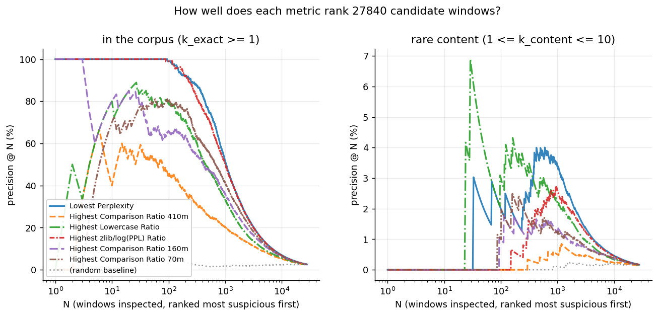The table above is five points on these curves. Every metric holds a plateau out to roughly the first 100 windows and then decays; the baseline stays flat at the bottom. The right panel is the same ranking scored against the rare set, where the best metric peaks below 7%.

This doesn’t align with the results from Carlini et al. and it is likely an artifact of the short size of the window.

It is actually very interesting to look from the other side: instead of asking how well perplexity ranks, we can group the windows by oracle hits k and look at the perplexity of each group.

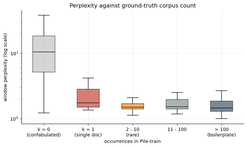
Confabulated windows (k = 0) sit higher than anything in corpus, which is why the ranking works at all. But the four in-corpus buckets are indistinguishable from each other: in this case perplexity is telling us if the model has likely seen a string, but not how often.

The side effect of using short windows

In our setting we rank 50-token windows instead of whole 256-token samples (which Carlini et al. did). So let’s try to “simulate” what 256-token windows would have changed.

Since a whole 256-token sample is basically never in the corpus, we take each metric’s top 100 samples, chop each into ~5 non-overlapping probes, and mark the whole sample as a hit if any probe is found in Pile-train.

metric	256-token windows	50-token windows	median distinct tokens	median compression
Lowest perplexity	41%	99%	0.11	0.18
Highest zlib/log(PPL) ratio	92%	99%	0.59	0.55
Lowest windowed perplexity	90%	—	0.56	0.57
Highest lowercase ratio	46%	79%	0.54	0.55
Highest comparison ratio (410m)	9%	45%	0.52	0.51

(Windowed perplexity is a sample-level metric: it has no 50-token column because a window has no sub-window to minimise over, which is also why it is absent from the table above.)

Most notably, in this settings the accuracy of raw perplexity as a predictor for memorization drops dramatically. This is expected as, the longer the sequence, the more likely it is for perplexity to converge.

In this case most other metrics surpass raw perplexity.

How much of the rare set is actually rare?

~90% of the rare (k_content <= 10) windows, are composite of parts more common than the whole.

k_content	k_part	window
4	1,217,684	`WITHOUT WARRANTIES OR CONDITIONS OF ANY KIND, either express or implie…`
6	193,977	`}); } }); }); }); <script src="https://ajax.googleapis.com/ajax/libs/j…`
1	181,727	`] }, { "cell_type": "code", "execution_count": 12, "metadata": {}, "ou…`
3	97,580	`AAAAAHHHHHHHHHHHHHHHHHHHHHHHHHHHHHHHHHHHHHHHHHHHHHHHHHHHH…`
2	48,309	`: "Summary judgment is proper when the pleadings, depositions, answers…`

These matches are memorized boilerplate.

What did the model actually memorize

Of the 47 rare windows, 43 have a sub-span at least 100x more common than the window itself. Here are the remaining:

k=2  k_part=2     ratio 1x    ' \n  3. 3. \n  4. 4. \n  5. 5. \n  6. 6. \n  7. 7. \n …'
k=6  k_part=566   ratio 94x   '\n#include "clang/Basic/Diagnostic.h"\n#include "clang/Stati…'
k=3  k_part=—     ratio n/a   '‚‚‚‚‚‚‚‚‚‚‚‚‚‚‚‚‚‚‚‚‚‚‚‚‚'
k=3  k_part=—     ratio n/a   '€‚‚‚‚‚‚‚‚‚‚‚‚‚‚‚‚‚‚‚‚‚‚‚‚'

The bottom two are repeated-character garbage. The second is a clang include block that almost hit our k_part threshold (94x against a 100x cut). The first is a blank worksheet from a knitting book.

Here is a selection of the other 43, sorted by how boilerplate-composed it is. Everything below is really in the corpus (infini-gram retrieved the document).

k	k_part	subset	extracted
1	719	Github	`WHATSOEVER RESULTING FROM LOSS OF MIND, USE, DATA OR PROFITS, WHETHER IN * AN ACTION OF CONTRACT…`
1	1,036	Github	`Denver and NAG Ltd..-- * April 2012 * * .. Scalar Arguments .. CHARACTER UPLO INTEGER INFO, LDA, N`
1	1,761	Pile-CC	`Foundation, Inc. The GNU C Library is free software; you can redistribute it and/or modify it…`
2	1,980	Github	`two APIs, API diff, Javadoc, doclet"> <TITLE> android.media.MediaCodec </TITLE> <link href="…`
3	2,593	Books3	`3. Title Page 4. Contents 5. Start 1. b 2. iii 3. iv 4. v 5. vii 6. viii 7.`
2	3,099	Books3	`Except in the United States of America, this book is sold subject to the condition that it shall not…`
8	6,930	FreeLaw	`COURT'S LOCAL RULE 32.1.1. WHEN CITING A SUMMARY ORDER IN A DOCUMENT FILED WITH THIS COURT, A PARTY…`
4	12,176	OpenWebText2	`Pelosi slams Trump executive order on pre-existing conditions: It 'isn't worth the paper it's…`
6	17,541	Github	`OUT_RETURN_TYPE = YES; GCC_WARN_UNINITIALIZED_AUTOS = YES; GCC_WARN_UNUSED_FUNCTION = YES;`
3	97,580	Pile-CC	`AAAAAHHHHHHHHHHHHHHHHHHHHHHHHHHHHHHHHHHHHHHHHHHHHHHHHHHHH…`
1	181,727	Github	`] }, { "cell_type": "code", "execution_count": 12, "metadata": {}, "outputs": [], "source": [ "sess`
4	1,217,684	Github	`WITHOUT WARRANTIES OR CONDITIONS OF ANY KIND, either express or implied. * See the License for the…`

The model mostly memorizes by repetition, so anything it holds firmly enough to regurgitate is something it saw thousands of times (and probably not worth extracting). What lands in the rare bucket got there by being structurally odd.

However 47 candidates out of ~28K is too thin to say anything about it.

Going after the secrets directly

In the previous sections we tried to mine any type of unstructured content with a focus on rare entries.

However, data extraction could be approached in several different ways. For instance, if we shrink our focus to short, structured (and very distinguishable) content (e.g. emails, URLs, phone numbers), our frame of reference changes.

Suddenly k_content is less relevant (content has a standard structure) and k_part no longer applies (content is short).

In this context the count changes of meaning:

k = 0: the model made it up
k small: real, and rare enough to be specific
k large: e.g. support@github.com, not interesting

Scanning the top samples for this type of content yields this:

type	counted	k = 0	in corpus	1 ≤ k ≤ 10	median k
email	381	356	25	0	672
url	400	281	119	18	766
phone-like	80	56	24	16	6
uuid / hex	44	42	2	0	2,194
base64-ish	22	22	0	0	—
PERSON	222	137	85	12	627
ORG	248	123	125	10	3,408

Two caveats on these numbers. The patterns over-match, so each row is an upper bound (ORG in particular absorbs a lot of class names). And counting is capped at 400 entities per type, which url, PERSON and ORG all hit (727, 2,691 and 3,017 unique were mined): those three rows are a deterministic sample, not a population total.

We extracted 25 email addresses, and the rarest occurs 22 times and lives in a Copyright header:

k=22     j*@hpl.hp.com              Github
k=26     s***********@fpl.com       Enron Emails
k=103    s******@enron.com          Enron Emails
k=128    s****@moshier.net          Github
k=672    b****@calpine.com          Enron Emails

We got some odd URLs which look genuinely rare:

k=1   http://localhost:2310/           Github
k=1   http://www.libreelec.tv          Github
k=2   http://www.meadowlark.com        ArXiv
k=4   http://www.cs.binghamton.edu/    ArXiv

The phone pattern mostly caught Texas appellate docket numbers NN-NN-NNNNN, fourteen of them, all at k <= 7 and half at k <= 2.

k=1   08-******31   FreeLaw        k=2   04-******95   FreeLaw
k=1   13-******96   FreeLaw        k=4   05-******24   FreeLaw
k=6   (71*********59   Enron Emails   <- the one real phone number

A docket points to one specific case. It is the closest thing to a record identifier this run produced.

We got only two real UUIDs, and one is the nil UUID:

k=25       FAE04EC0-301F-11D3-BF4B-00C04F79EFBC     
    StackExchange, Github
k=2,194    00000000-0000-0000-0000-000000000000    OpenWebText2, StackExchange

The names (which we extracted using spaCy NER) are mostly ordinary people from crawled pages:

k=1   C. M*** W****        Pile-CC
k=1   J***** A********     Pile-CC
k=1   MARK K******         FreeLaw
k=4   M****** P. W*****    Wikipedia (en), FreeLaw
k=2   Mayberry Rules       Pile-CC     <- not a person

Does this work on closed-weights models?

We attacked an open-weights model, but nothing in the attack fundamentally needs the weights, only token logprobs. And since the candidates are the model’s own generations, an API that returns the logprob of each sampled token gives us the perplexity of every sample for free, as a by-product of step 1. That is enough for raw perplexity, windowed perplexity and the zlib ratio; the comparison ratio also works, since the second estimate comes from a small model we run locally.

The real obstacles are elsewhere:

unconditional sampling from assumes access to a base model, an aligned model might not play along in the same way
generating hundred thousands samples through an API costs real money and bumps into rate limits
without the training corpus, verification goes back to being application-specific

Conclusion

Generate-then-rank does work: out of ~120K samples, 708 deduplicated 50-token windows are verbatim in Pile-train, and every ranking metric beats the random baseline by a wide margin. But almost everything we pulled out is boilerplate.

In practice:

Verification is the hard part, not generation. A naive count is not enough, k_content (re-renderings) and k_part (sub-spans) often tell a different story.
Ranking metrics are sensitive to what you rank. Raw perplexity dominated on 50-token windows and collapsed to 41% on 256-token samples.
Repetition-driven memorization is not very interesting to extract. What a 1.4B model holds firmly enough to regurgitate is mostly common text.
Narrowing the target helps. Verification is easier than for unstructured text, and we were able to extract a few rare URLs, Texas appellate docket numbers and one real phone number.

Things worth trying

Better seeding. Special-Characters Attack (Bai et al., 2024): structural symbols like {, }, @ and # co-occur heavily with structured training data (JSON, emails, code) and act as stronger memory triggers than words.
Aggregate the metrics instead of comparing them. We deliberately kept one ranking per metric to measure them; a combined score (or a small classifier over all of them) should rank better than any single one.
Scale and model size. 47 rare windows is far too thin to conclude anything about what gets memorized. More samples, and the larger Pythia checkpoints, would both help (memorization grows with capacity).
And much more…this was just a simple proof-of-concept experiment after all :)

This lab was entirely about extractability. That is only one face of memorization. In future labs I plan to explore other angles.

The code

The full notebook for this lab is here: Data Extraction Lab 2 (Colab).

AI Security

AI Data Extraction Privacy

This post is licensed under CC BY 4.0 by the author.